An artificial neural network (ANN) is a type of machine learning model. It is made up of a number of simple parts called units, or neurons. By combining a large amount of these simple units, ANNs can solve real-world problems. For example, the main network that was used in my bachelor thesis research consisted of over 12,000 units. The name artificial neural network is slightly misleading: they’re mostly related to biological neural networks through the fact that both artificial and natural neural networks are made up of simple parts. Other than that they’re quite unrelated.
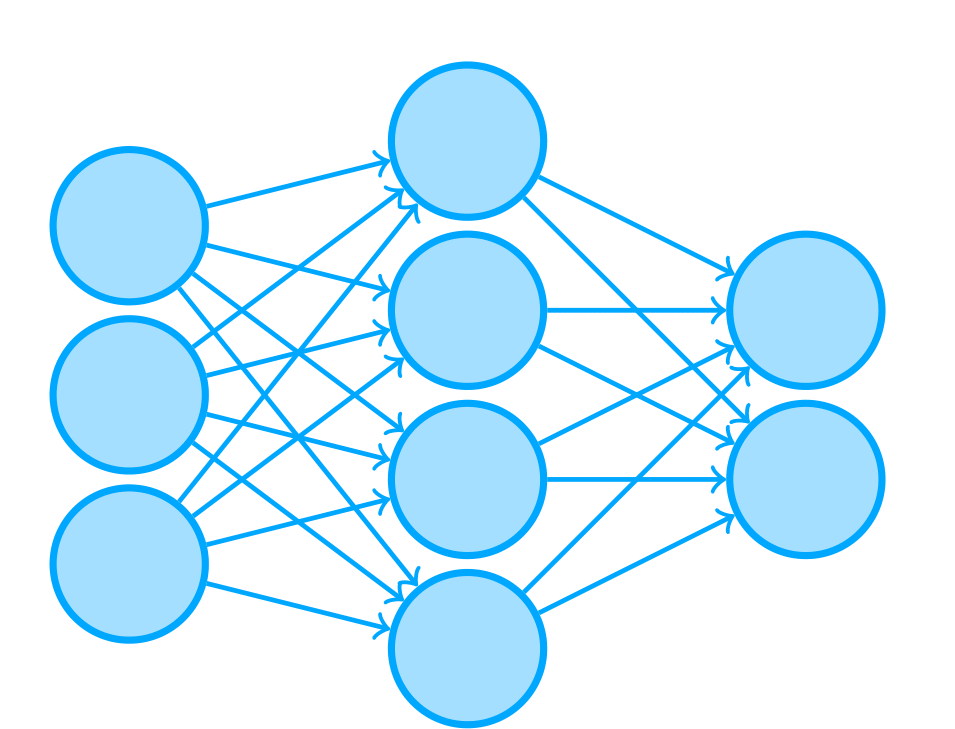
A simple ANN
The power of neural networks comes from the connections between units. These can be weighted, such that some connections are more important than others. To get the network to calculate something, some of the units are activated by a certain value. These units then activate or deactivate the units that are connected to them. For most practical purposes, a network has a clear set of units that act as the input and a clear set of units that act as the output. For example, the inputs to the network shown above are the units on the left. The next layer of units that are connected to the first layer calculate their activations based on the first layer. Finally, the units in the output layer calculate their activations based on the second layer.
Units
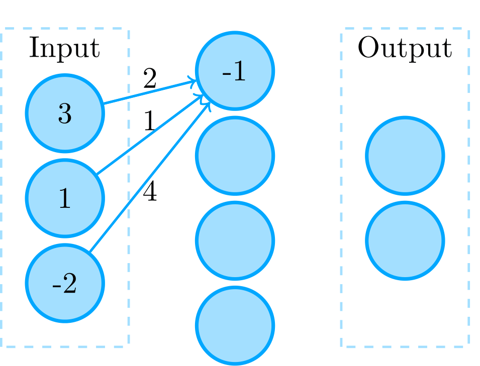
An ANN; the calculation of one unit’s activation can be seen
Each unit is very simple; it just has a certain numeric activation value. For the input units the activation is set to known values; in the case of a network used for image processing the input units’ activations could correspond to an image’s pixel values. The other units calculate their activation values as a function of their input activations, which are based on the units they are connected to and the weights of those connections. For example, the activation function of the unit that can be see in the figure on the right is f(x) = x with as input activation x = 2 \cdot 3 + 1 \cdot 1 + 4 \cdot -2 = -1. In general, when working with layered networks like this you call layer l the input for layer l+1. For example, the middle layer here is the input for the last (output) layer.
Network activations can be efficiently computed by using parallelization. To do this in MATLAB, you generally represent units as vectors and the connections as weight matrices. Here, the network input would be the vector:
and the weight matrix of the middle layer could be:
Then, the activations of the middle layer are calculated as the matrix-vector product \mathbf{y} = \mathbf{W} \mathbf{x}. Thus:
Generally, an activation function f is applied entrywise to the calculated activations, such that the output becomes:
In general, one wants this activation function to be non-linear. This is especially important in multi-layered networks, as adding multiple layers with a linear activation function has no added power over a larger single-layered (input-output) network. This is because each layer’s output values – the vector \mathbf{y} – can be calculated as the linear matrix-vector product of the layer’s weights and input. If f is, for example, f(x)=x, the full output of a network can be calculated simply by multiplying its weight matrices to obtain the combined weight matrix:
By using a non-linear activation function f, this property does not hold. In effect, the network is able to learn non-linear representations of the input. Often used non-linear activation functions are the sigmoid function f(x) = \frac{1}{1 + e^{-x}} and the rectified linear unit f(x) = \max \left(x, 0\right).
Besides these weights, a unit can have a bias which is its intrinsic tendency to be activated. Thus, a layer’s full output becomes:
Training
These networks are not inherently useful. They are trained by giving them large amounts of example inputs, such as images belonging to different classes. For each example the network performs its calculation and gives a certain output. In the early stages this output is generally wrong. You then calculate how the connection weights have to be changed such that the network would have provided a better answer. For multi-layered networks this is often done by utilizing gradient descent and backpropagation. This is repeated many times, with the goal to create a network that gives accurate answers to the inputs. If successful, such a network should be able to be generalized for use on unseen inputs.
Training an ANN with gradient descent and backpropagation is performed by optimizing an objective function. In order to update the weights and biases of layers the gradients of the objective function value with respect to the weights and biases have to be known for those layers. This is achieved by iteratively propagating the gradient known in layer l back to layer l-1, starting from the top layer. If the error E is the scalar output of the objective function, then the error gradient with respect to a certain layer’s weights \mathbf{W_l} can be computed by using the chain rule.
Here, L is the number of layers in the network and \mathbf{w_l} is the vectorized weight matrix of layer l. Practically, to calculate the gradient for a weight matrix \mathbf{W} the gradient of the error with respect to its output \mathbf{y} has to be known; \partial E/\partial \mathbf{y}. This gradient is given by the layer above through its calculation of the gradient of the error with respect to its input; \partial E/\partial \mathbf{x'}. As follows from the network’s architecture \mathbf{x'} := \mathbf{y} and thus \partial E/\partial \mathbf{y} = \partial E/\partial \mathbf{x'}. For the objective function, the topmost “layer”, \partial E/\partial \mathbf{y} = 1, as E is defined as the output of the objective function. The gradient can then be propagated back through the layers by repeatedly calculating \partial E/\partial \mathbf{x}. To update weights \mathbf{W} and biases \mathbf{b} of a layer, \partial E/\partial \mathbf{W} and \partial E/\partial \mathbf{b} can be calculated. For biases \mathbf{b}, and vectorized weights \mathbf{w} = \text{vec}(\mathbf{W}):
Once the gradient of the error with respect to layer weights and biases are known, they can be updated in direction opposite to the gradient to improve network performance. The simplest update routine is performing a small step in direction of the negative gradient.
Here, \eta is the learning rate, and \mathbf{W}' and \mathbf{b}' are the new weights and biases.
Types of Networks
There are various different types of ANNs. Many can be described as being deep neural networks, which are networks that consist of multiple layers. The training of these networks has been laid out above. One remarkable such network is the convolutional neural network, where units correspond to specific receptive fields sensitive to overlapping parts of the input. ANNs can also be recurrent, meaning that the connections form a cycle (e.g., unit A activates unit B, which activates unit C, which activates unit A). One such network is the Hopfield network, which can store input patterns in its weights and reconstruct those patterns from (partial) inputs.